Integration
- The process of approximating a definite integral
using a numerical method is called quadrature - The Riemann sum suggests how to perform quadrature
![]()
- We will examine more accurate/efficient quadrature methods

Integration
- Quadrature also generalizes naturally to higher dimensions,
and allows us to compute integrals on irregular domains - For example, we can approximate an integral on a triangle
based on a finite sum of samples at quadrature points![]()
![]()
![]()
people.sc.fsu.edu/~jburkardt/cpp_src/triangle_fekete_rule_test


Integration
- And then evaluate integrals in complex geometries
by triangulating the domain

ODEs: IVP
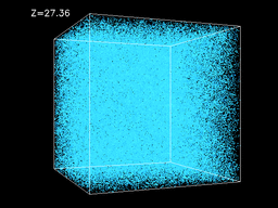
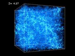
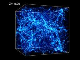
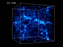
- $N$-body problems are the basis of many cosmological simulations
- Recall the galaxy formation simulations from Unit 0
![]()
![]()
![]()
![]()
- Computationally expensive when $N$ is large!
ODEs: BVP
- We can approximate the equation $-u''(x) = f(x)$ with finite differences \[ -\frac{u(x+h) -2u(x) + u(x-h)}{h^2} = f(x) \] and impose $u(-1) = 0$ and $u(1) - u(1 - h) = 0$

PDEs
- Again, we can approximate the equation $\frac{\partial u}{\partial t} - \frac{\partial^2 u}{\partial x^2} = f(x)$
with finite differences \[ \textstyle \frac{u(x,t)-u(x,t-\Delta t)}{\Delta t}-\frac{u(x+h,t) -2u(x,t) + u(x-h,t)}{h^2} = f(x) \] and impose $u(x,0)=0$, $u(-1,t) = 0$, and $u(1,t) - u(1 - h,t) = 0$

PDEs
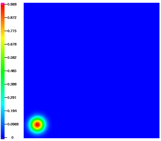
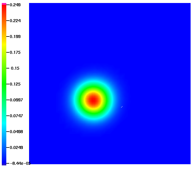
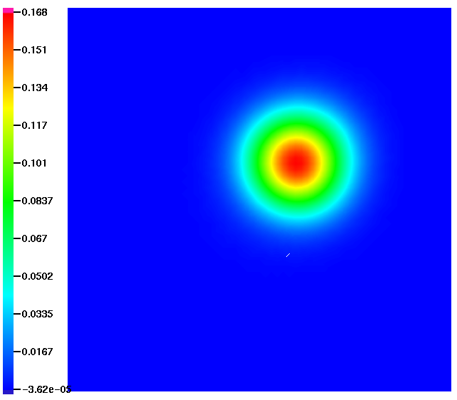
- We can add a transport term to the heat equation
to obtain the convection-diffusion equation
\[ \frac{\partial u}{\partial t} + \mathbf{w}\cdot\nabla u - \nabla^2 u = f(x,y) \] - Now $u(x,t)$ models the concentration of some substance
in a medium moving with velocity $\mathbf{w}(x,y,t)\in\mathbb{R}^2$![]()
![]()
![]()
PDEs
- Numerical methods for PDEs are a major topic in scientific computing
- Recall examples from Unit 0
![]()
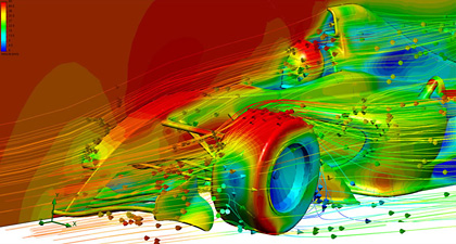
CFD![]()
Geophysics - In the course, we will focus on the finite difference method
- Alternative methods: finite element, finite volume,
spectral, boundary element, particles, …
Runge Phenomenon Again
- Answer: In the constant $C_n$
- Recall that $C_n = b-a + \sum_{k=0}^n|w_k|$, and that $w_k = \int_a^b L_k(x) \text{d}x$
![]()
- If the $L_k$ blow up due to equally spaced points, so does $C_n$

Gauss Quadrature
- Legendre polynomials satisfy a recurrence relation \[ \begin{aligned} P_0(x) &= 1\\ P_1(x) &= x\\ (n+1)P_{n+1}(x) &= (2n+1)xP_n(x) - nP_{n-1}(x) \end{aligned} \]
- The first six Legendre polynomials
![]()

Gauss Quadrature
- We can find the roots of $P_n(x)$ and derive the $n$-point
Gauss quadrature rule in the same way as for Newton–Cotes:
integrate the Lagrange interpolant - Gauss quadrature rules have been extensively tabulated for $x \in [-1,1]$
Number of points Quadrature points Quadrature weights 1 0 2 2 $-1/{\sqrt{3}}, 1/{\sqrt{3}}$ $1, 1$ 3 $-\sqrt{3/5}, 0, \sqrt{3/5}$ $5/9, 8/9, 5/9$ … … … - Key point: Gauss quadrature weights are always positive,
so Gauss quadrature converges as $n\to \infty$Gauss Quadrature Points
- Points cluster toward $\pm 1$ which prevents Runge’s phenomenon!
![]()
![]()
![]()
![]()
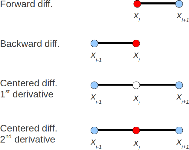
Finite Difference Stencils
- The pattern of points involved in a finite difference
approximation is called a stencil - Examples of stencils, $x_i$ is the point of interest
![]()
Example: Differentiation Matrix
- Forward difference corresponds to a bidiagonal matrix
with elements $D_{ii} = -\frac{1}{h},\;D_{i,i+1} = \frac{1}{h}$>>> import numpy as np >>> import matplotlib.pyplot as plt >>> n = 11 >>> h = 1 / (n - 1) >>> D = np.diag(-np.ones(n) / h) + np.diag(np.ones(n - 1) / h, 1) >>> plt.spy(D) >>> plt.show()
![]()
Example: Differentiation Matrix
- But the last row is incorrect,
$D_{n,n+1} = \frac{1}{h}$ is ignored!
![]()
Example: Differentiation Matrix
- Boundary points need different formulas
- For example, use the backward difference in the last row
$D_{n,n-1} = -\frac{1}{h},\;D_{nn} = \frac{1}{h}$![]()
- See [examples/unit3/diff_matr.py]
Example: A Predator–Prey Model
- The Lotka–Volterra equation is a two-variable nonlinear ODE
that models the evolution of populations of two species \[ y' = \left[ \begin{array}{c} y_1(\alpha_1 - \beta_1 y_2) \\ y_2(-\alpha_2 + \beta_2 y_1) \end{array} \right] \equiv f(y) \] - Unknowns are the populations $y_1$ (prey) and $y_2$ (predator)
- Parameters are $\alpha_1$ (birth rate), $\alpha_2$ (death rate), $\beta_1$, and $\beta_2$ (interactions)
- See [examples/unit3/lotka_volterra.py]
![]()
Example: ODE Stability
- Stability of $y' = \lambda y$ for different values of $\lambda$
- solution $y= y_0 e^{\lambda t}$ for $y_0=1$
- perturbed solution $\hat{y}= \hat{y}_0 e^{\lambda t}$ for $\hat{y}_0=0.9$
- difference $|\hat{y}-y|= |\hat{y}_0-y_0| e^{\lambda t}$

$\lambda = -1$
asymptotically stable
$\lambda = 0$
stable
$\lambda = 1$
unstableStability: Forward Euler
- Therefore, forward Euler is stable for $h\lambda \in \mathbb{C}$
inside the circle of radius 1 centered at $(-1,0)$ - This is a subset of the left-half plane $\mathrm{Re}(h\lambda) \leq 0$
![]()
- We say that the forward Euler method is conditionally stable:
if $\mathrm{Re}(\lambda) \leq 0$, we have to restrict $h$ to ensure stability
Stability: Backward Euler
- Let $h\lambda = a + ib$, then $1^2 \leq |1-(a+ib)|^2$, i.e. $(1-a)^2 + b^2 \geq 1$
![]()
- If Re$(\lambda) \leq 0$, this is satisfied for any $h > 0$
- We say that the backward Euler method is unconditionally stable:
if $\mathrm{Re}(\lambda) \leq 0$, no restriction on $h$ for stability
Stability Regions
ODE
$y'=\lambda y$
$y(t) = y_0 e^{\lambda t}$
$|e^{\lambda}| \leq 1$
forward Euler
$y_{k+1}=y_k+h\lambda y_k$
$y_k=y_0 (1+h\lambda)^k$
$|1+h\lambda|\leq1$
backward Euler
$y_{k+1}=y_k+h\lambda y_{k+1}$
$y_k=y_0 / (1-h\lambda)^k$
$|1 /(1-h\lambda)|\leq1$
Runge–Kutta Methods: Stability
- Stability regions of $p$-stage Runge–Kutta methods of order $p$
(do not depend on a particular method)
![]()
Higher-Order Methods: Stability
- Stability region of Fehlberg’s order 7 method (13 stages)
compared to order $p$ Runge–Kutta methods
![]()
Shooting Method: Example
- Steady-state diffusion-reaction equation ($\alpha=1, \gamma=-5$) \[ -\alpha u''(x) + \gamma u(x) = 0,\quad x\in[0,1] \]
- Dirichlet conditions: $u(0)=0$ and $u(1)=0.5$
and extra Neumann condition: $u(0)=g$ - Iteration: $g_\text{new} = g + \eta(0.5 - u(1))$ with $\eta=2$
![]()
- See [examples/unit3/shooting.py]
PDEs: Hyperbolic
- Wave equation: $u_{tt} - u_{xx} = 0$
- Corresponding quadratic function is $q(x,t) = t^2 - x^2$
- $q(x,t) = c$ gives a hyperbola, e.g. for $c=0,2,4,6$, we have
![]()
PDEs: Parabolic
- Heat equation: $u_{t} - u_{xx} = 0$
- Corresponding quadratic function is $q(x,t) = t - x^2$
- $q(x,t) = c$ gives a parabola, e.g. for $c=0,2,4,6$, we have
![]()
PDEs: Elliptic
- Poisson equation: $u_{xx} + u_{yy} = f$
- Corresponding quadratic function is $q(x,y) = x^2 + y^2$
- $q(x,y) = c$ gives an ellipse, e.g. for $c=0,2,4,6$, we have
![]()
Hyperbolic PDEs
- This tells us that the equation transports (or advects)
the initial condition with “speed” $c$\[ u_t + cu_x = 0 \]
- For example, with $c=1$ and an initial condition $u_0(x) = e^{-(1-x)^2}$
![]()
Characteristics
- Hence $u(X(t),t) = u(X(0),0) = u_0(X_0)$,
i.e. the initial condition is transported along characteristics - Characteristics have important implications for the direction of
flow of information, and for boundary conditions
$c>0$, must impose BC at $x=a$
cannot impose BC at $x=b$
$c<0$, must impose BC at $x=b$
cannot impose BC at $x=a$
Example: Variable Speed in Space
- Equation: $u_t+cu_x=0$ with $c(x,t) = x - 1$
- Characteristics satisfy $X'(t)=c(X(t), t)$
with solution $X(t) = 1 + (X_0 - 1)e^{t}$ - Characteristics “bend away” from $x=1$
![]()
Example: Variable Speed in Time
- Equation: $u_t+cu_x=0$ with $c(x,t) = t - 1$
- Characteristics satisfy $X'(t)=c(X(t), t)$
with solution $X(t) = X_0 + \tfrac{1}{2}t^2 - t$ - The same shape shifted along $x$
![]()
Hyperbolic PDEs: Numerical Approximation
- We impose an initial condition and a boundary condition
- A finite difference approximation is performed on a grid in the $xt$-plane
![]()
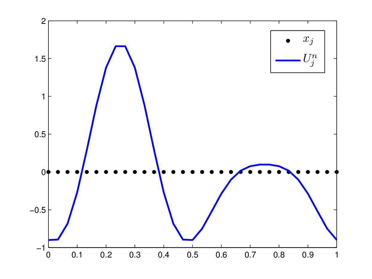
Hyperbolic PDEs: Numerical Approximation
- The set of grid nodes on which $U_j^{n+1}$ depends
is called the domain of dependence of $U_j^{n+1}$![]()
Hyperbolic PDEs: Numerical Approximation
- Domain of dependence of $U_j^n$: grid nodes •
- Domain of dependence of $u(t_{n+1}, x_j)$: solid line (characteristic)
![]()
- In this case, the scheme satisfies the CFL condition
Hyperbolic PDEs: Numerical Approximation
- With a larger advection speed $c$,
the scheme does not satisfy the CFL condition![]()
Hyperbolic PDEs: Numerical Approximation
- With a negative advection speed ($c<0$),
the scheme does not satisfy the CFL condition![]()
Hyperbolic PDEs: Numerical Approximation
- If $c > 0$, then we require $\nu = \frac{c\Delta t}{\Delta x} \leq 1$
for the CFL condition to be satisfied![]()
Hyperbolic PDEs: Central Difference
- Another method that seems appealing is the central difference method
\[
\frac{U_j^{n+1} - U_j^n}{\Delta t} + c \frac{U_{j+1}^{n} - U_{j-1}^n}{2 \Delta
x} = 0
\]
![]()
- It satisfies CFL for $|\nu| = |c\Delta t / \Delta x| \leq 1$ both for $c>0$ and $c<0$
- However, we will see that this method is unstable
Hyperbolic PDEs: Stability
- Suppose that $U^n_j$ is periodic on a grid $x_1,x_2,\ldots, x_n$
![]()
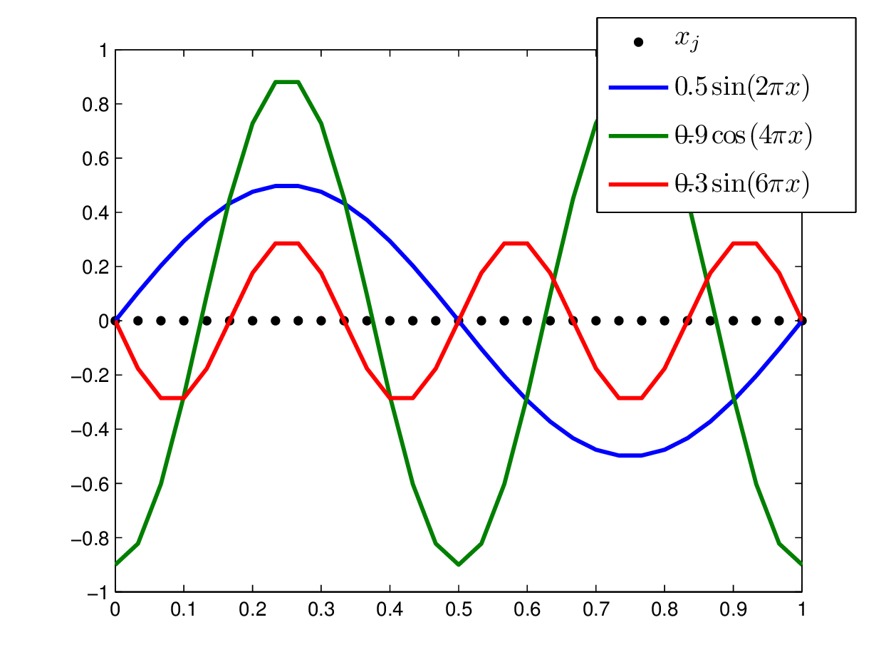
Hyperbolic PDEs: Stability
- Then we can represent $U^n_j$ as a linear combination
of $\sin$ and $\cos$ functions, i.e. Fourier modes![]()
- Equivalently, as a linear combination of complex exponentials,
since $e^{i kx} = \cos(kx) + i\sin(kx)$ so that \[ \textstyle \sin(x) = \frac{1}{2i}(e^{ix} - e^{-ix}), \qquad \cos(x) = \frac{1}{2}(e^{ix} + e^{-ix}) \]
Wave Equation: Example 🔊
- Wave equation with forcing
\[
u_{tt} - u_{xx} = f
\]
![]()
- Energy $\int{u_t^2dx}$
- Sound $\int{u_x^2dx}$ (change in arc length)
- Forcing $f = x \sin(\omega(t) t)$
$\omega(t)=at + b$
$\theta$-Method: Stability
- Note that this corresponds to the highest frequency mode
that can be represented on our grid, since with $k = \pi/\Delta x$ we have \[ e^{ik(j\Delta x)} = e^{\pi i j} = (e^{\pi i})^j = (-1)^j \] - The $k = \pi/\Delta x$ “sawtooth” mode
![]()
$\theta$-Method: Stability
- The $\theta$-method is conditionally stable if $\theta\in[0, 0.5)$
and unconditionally stable if $\theta\in[0.5, 1]$ - Stability region in the $\mu$-$\theta$ plane
![]()
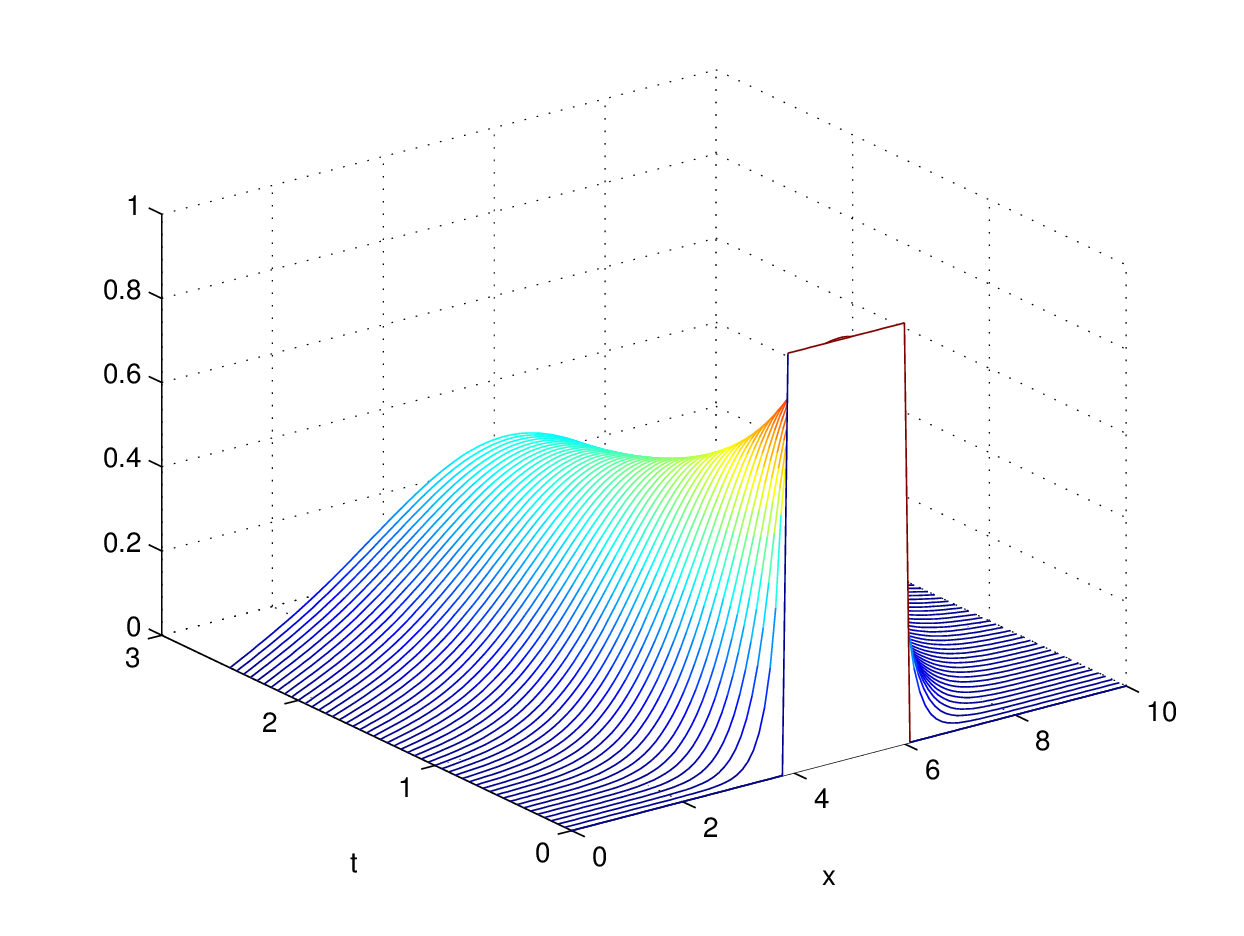
Heat Equation
- Note that the heat equation describes a diffusive process,
so it tends to smooth out discontinuities - See [examples/unit3/heat.py],
forward Euler and Crank-Nicolson schemes for the heat equation![]()
- This is qualitatively different to hyperbolic equations,
e.g. the advection equation will just transport a discontinuity in $u_0$
Elliptic PDEs
- We will consider how to use a finite difference scheme
to approximate this 2D Poisson equation - First, introduce a uniform grid to discretize $\Omega$
![]()
Elliptic PDEs
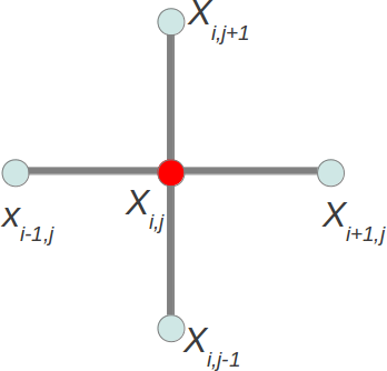
- Using the grid values, the approximation to the Laplacian is \[ u_{xx} + u_{yy} \approx \frac{U_{i,j-1} + U_{i-1,j} - 4U_{i,j} + U_{i+1,j} + U_{i,j+1}}{h^2} \]
- This corresponds to a 5-point stencil
![]()
Elliptic PDEs
- For instance, let’s enumerate the nodes from 0 to $N_xN_y-1$
starting from the bottom row $j=0$ (i.e. row-major order)![]()
- Let $G$ denote the mapping from the 2D indexing to the 1D indexing
- From the above schematic we have \[ G(i,j) = jN_x + i \quad \text{and therefore} \quad U_{G(i,j)} = U_{i,j} \]
Elliptic PDEs
- For example, in the case $N_x = N_y = 6$,
matrix $D$ has the following sparsity pattern![]()
Elliptic PDEs
- Poisson equation $\nabla^2 u = -10$
for $(x,y) \in \Omega = [0,1]^2$ with $u = 0$ on $\partial \Omega$![]()
- See [examples/unit3/poisson.py], solved using
scipy.sparse
- Key point: Gauss quadrature weights are always positive,